Earth observation guideApplications
Forestry
Forests are large, remote and slow to survey on foot. From orbit their loss, regrowth, height and carbon can be measured consistently over decades.
The basics
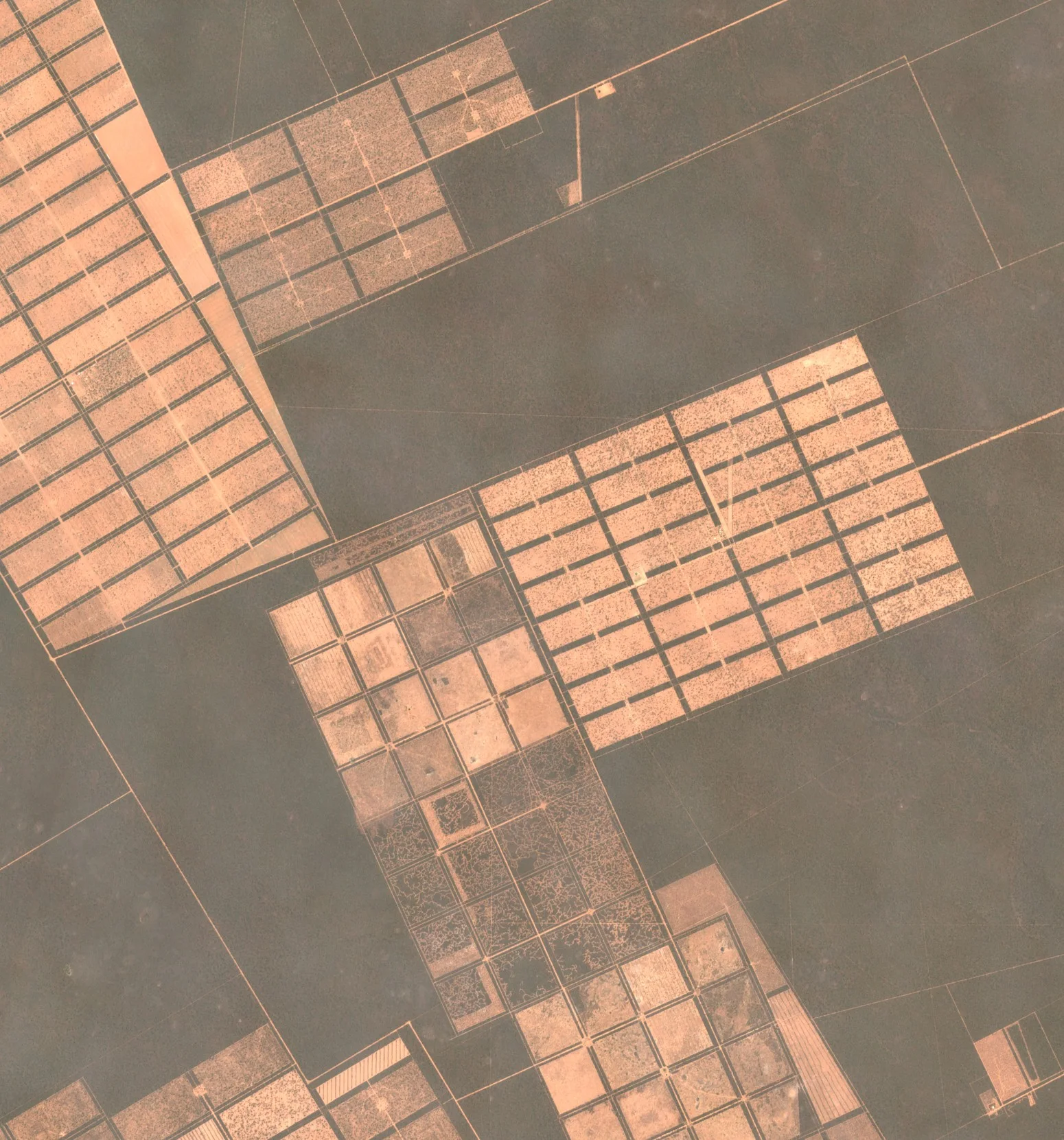
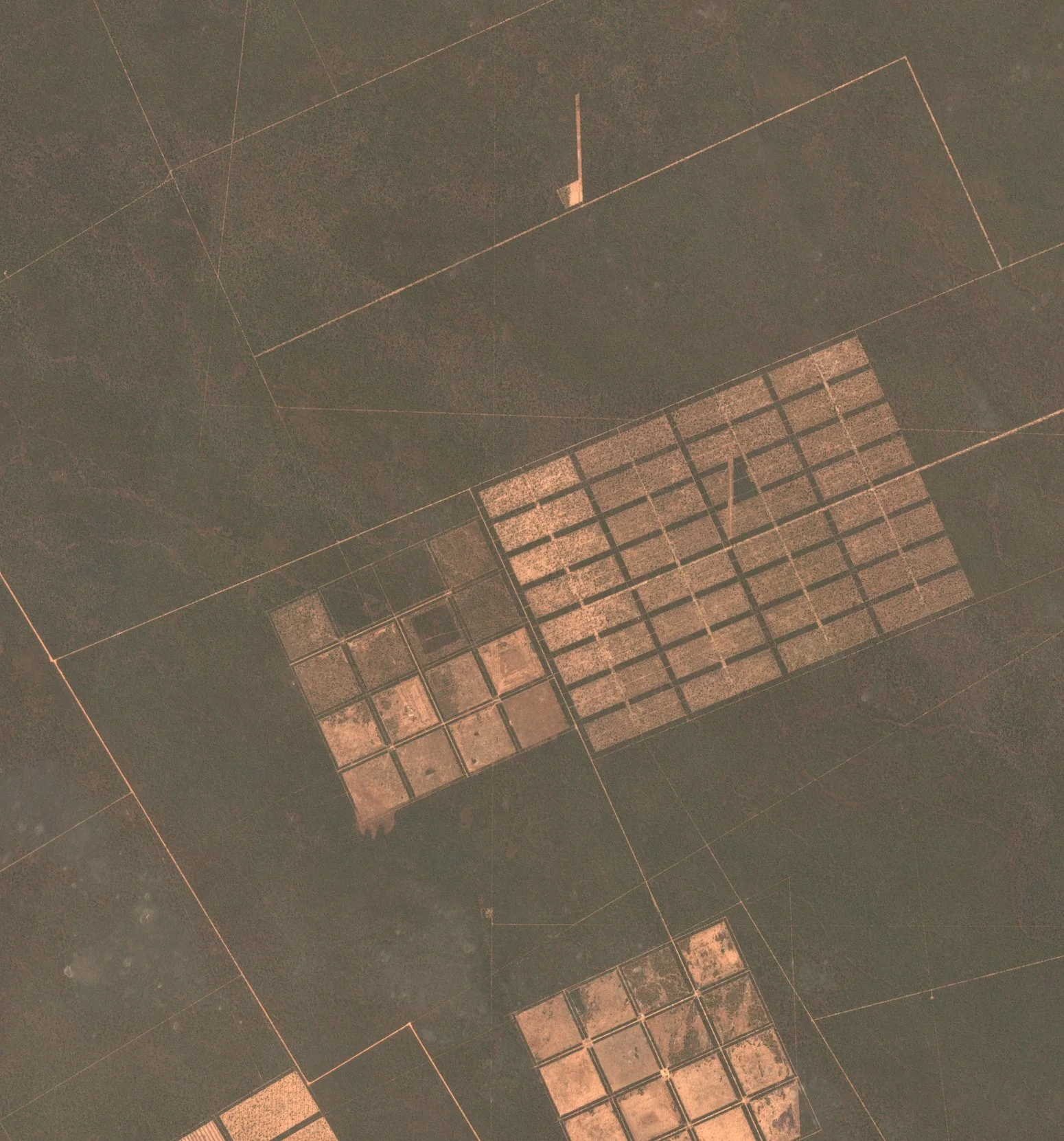
Walking a forest to count and measure its trees takes a team weeks, and most forests are never walked at all. Satellites look at all of them, year after year. They show where trees have been felled, burnt or blown down, and how quickly they grow back. With height measurements added, they help estimate how much timber or carbon a forest holds. Forest owners use this to plan harvests, governments to enforce the law, and companies to show that the wood, soya or beef they buy did not come from land that was recently forest.
Why it matters
Forests store carbon, shelter wildlife and supply timber, and losing them is hard to undo. Rules on deforestation-free products and carbon markets both depend on knowing where forest stood and when it was cleared, and only satellite records go back far enough and cover enough ground.
In depth
Forest monitoring uses almost every kind of data in this guide. Multispectral time series map where canopy has gone, radar keeps watching through tropical cloud and senses woody structure, and elevation data from laser scanning or radar give height. Longer radar wavelengths reach deeper into the canopy, which is why biomass missions use them [1].
Forest cover change
Satellite time series were used to map global forest loss of 2.3 million square kilometres and gain of 0.8 million square kilometres between 2000 and 2012 at a resolution of 30 m. The tropics were the only climate domain with a trend, with loss rising by 2,101 square kilometres a year, and the falling rate of deforestation in Brazil was offset by rising loss in countries including Indonesia, Malaysia, Paraguay and Bolivia [2].
- What is measured
- Whether each pixel holds tree cover, and the year in which cover was lost or gained.
- Data
- Multispectral archives at 10 to 30 m, processed into consistent annual layers.
- How often
- Annual maps, built from every usable image in the year.
- Limits
- Gradual thinning and degradation are harder to see than clearing. Plantations and natural forest can look alike, so loss and gain are not the same as deforestation and reforestation.
- Who uses it
- Governments reporting on forests and climate, researchers, campaign groups and companies screening their supply chains.
Disturbance alerts
An annual map arrives too late to stop illegal felling, so alert systems flag new disturbance as each image arrives. A Landsat-based alert for humid tropical forest was issued weekly in Peru, the Republic of Congo and Kalimantan, and in Peru it was found to have very high user's accuracy, which makes it a conservative product suited to land management and enforcement [3]. Radar avoids the cloud that delays optical alerts. A Sentinel-1 alert for the Congo Basin, with observations every 6 to 12 days at 10 m, mapped 4 million disturbance events totalling 1.4 million hectares between January 2019 and July 2020. Nearly 80 per cent were smaller than half a hectare, and events of 0.2 hectares and larger were detected confidently [4].
- What is measured
- A sudden drop in optical greenness or in radar backscatter, compared with the history of the same pixel.
- Data
- Radar at 10 to 20 m where cloud is frequent, and multispectral imagery at 10 to 30 m. Finer optical images confirm an alert.
- How often
- Each new image, which means days to a couple of weeks.
- Limits
- The smallest clearings, and selective logging under an intact canopy, can be missed. Each alert needs confirming before action is taken.
- Who uses it
- Forest agencies and police, protected area managers, and companies checking that the farms they buy from have not cleared land.
Biomass, height and carbon
Carbon accounting for a forest starts with its above-ground biomass, the dry mass of the living wood and leaves. Combining several radar backscatter datasets from around 2010 gave a global map of forest above-ground biomass at 1 hectare, checked against 110,897 field plots, with a total of 522 petagrams. The map is less certain in forests holding more than 250 megagrams per hectare [5]. The European Space Agency's BIOMASS mission was designed for exactly this measurement, its primary objective being the worldwide distribution of forest above-ground biomass [6]. Height is the other half of the picture. A deep learning model that fused sparse spaceborne laser heights with Sentinel-2 images produced a global canopy height map at 10 m for 2020, which found that only 5 per cent of the land is covered by trees taller than 30 m [7].
- What is measured
- Radar backscatter and canopy height, related to field-measured biomass and from that to carbon.
- Data
- Long-wavelength radar, elevation and canopy height models, and multispectral images to map them across the land.
- How often
- Usually one map every year or few years.
- Limits
- Maps are least certain in the densest, highest-biomass forests, and every map depends on field plots for calibration and checking.
- Who uses it
- Carbon project developers and verifiers, national greenhouse gas inventories and climate scientists.
Forest inventory
Managers planning a harvest need stand-level figures for height, volume and species. A review of four technologies for forest inventory identified airborne laser scanning as transformative, with terrestrial laser scanning, digital aerial photogrammetry and high resolution satellite imagery as the others with the greatest potential [8]. Satellite data extend a laser survey across a whole estate and keep it current between surveys.
- What is measured
- Canopy height, tree crowns, species groups and the volume derived from them.
- Data
- Elevation from laser scanning or stereo images, very high resolution optical imagery and multispectral or hyperspectral data for species.
- How often
- A full inventory every few years, updated with satellite images in between.
- Limits
- Laser surveys are costly, and species and stem counts still need field plots.
- Who uses it
- Forest owners and managers, timber buyers and certification bodies.
Fire and burn severity
Burnt ground is dark in the near infrared and bright in the shortwave infrared, the opposite of green vegetation, so the normalised burn ratio built from the two bands drops sharply after a fire. The difference between the ratio before and after a fire measures how severe it was. A relative version of that difference adjusts for how much vegetation there was before the fire, so that severity can be compared across very different landscapes [9].
- What is measured
- The change in near and shortwave infrared reflectance from before to after a fire.
- Data
- Multispectral imagery with shortwave infrared bands at 10 to 30 m, and thermal data for active fires.
- How often
- One image before and one soon after the fire, then repeated to follow recovery.
- Limits
- Smoke and cloud can hide the scar for days, and a low-intensity fire under the canopy may barely register.
- Who uses it
- Forest and land managers planning restoration, and insurers assessing losses.
23 August 2017
26 September 2023
References
- Woodhouse, I. H. (2017) Introduction to Microwave Remote Sensing. CRC Press. https://doi.org/10.1201/9781315272573
- Hansen, M. C., Potapov, P. V., Moore, R. et al. (2013) High-Resolution Global Maps of 21st-Century Forest Cover Change. Science, 342(6160), 850-853. https://doi.org/10.1126/science.1244693
- Hansen, M. C., Krylov, A., Tyukavina, A. et al. (2016) Humid tropical forest disturbance alerts using Landsat data. Environmental Research Letters, 11(3), 034008. https://doi.org/10.1088/1748-9326/11/3/034008
- Reiche, J., Mullissa, A., Slagter, B. et al. (2021) Forest disturbance alerts for the Congo Basin using Sentinel-1. Environmental Research Letters, 16(2), 024005. https://doi.org/10.1088/1748-9326/abd0a8
- Santoro, M., Cartus, O., Carvalhais, N. et al. (2021) The global forest above-ground biomass pool for 2010 estimated from high-resolution satellite observations. Earth System Science Data, 13(8), 3927-3950. https://doi.org/10.5194/essd-13-3927-2021
- Quegan, S., Le Toan, T., Chave, J. et al. (2019) The European Space Agency BIOMASS mission: Measuring forest above-ground biomass from space. Remote Sensing of Environment, 227, 44-60. https://doi.org/10.1016/j.rse.2019.03.032
- Lang, N., Jetz, W., Schindler, K. and Wegner, J. D. (2023) A high-resolution canopy height model of the Earth. Nature Ecology & Evolution, 7(11), 1778-1789. https://doi.org/10.1038/s41559-023-02206-6
- White, J. C., Coops, N. C., Wulder, M. A. et al. (2016) Remote Sensing Technologies for Enhancing Forest Inventories: A Review. Canadian Journal of Remote Sensing, 42(5), 619-641. https://doi.org/10.1080/07038992.2016.1207484
- Miller, J. D. and Thode, A. E. (2007) Quantifying burn severity in a heterogeneous landscape with a relative version of the delta Normalized Burn Ratio (dNBR). Remote Sensing of Environment, 109(1), 66-80. https://doi.org/10.1016/j.rse.2006.12.006